Modern Robotics Capstone Project | Coursera Specialization
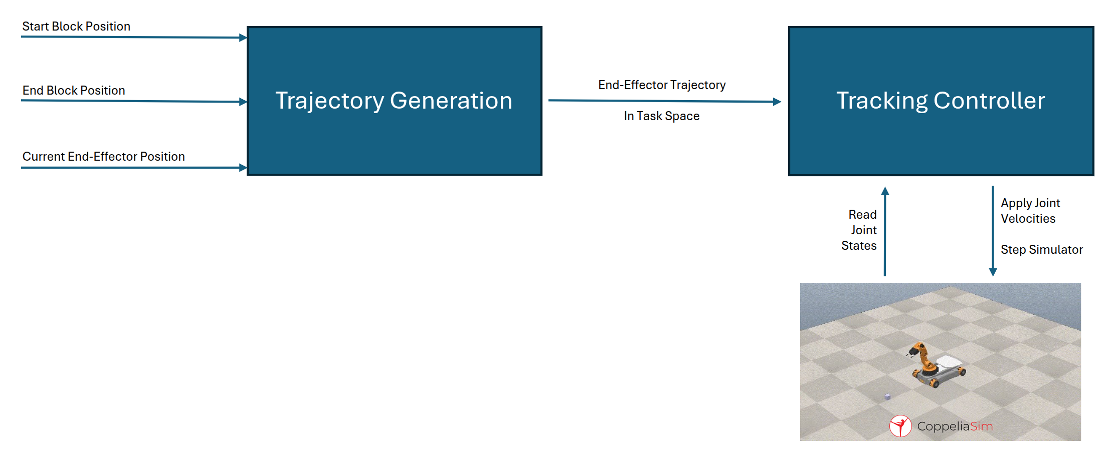
This project involved developing a pick-and-place pipeline for a Kuka Youbot Robot in fulfillment of the Modern Robotics Coursera specialization. The pipeline takes as input the current position of the block in the world and the desired placement position of the block, generates a simple end-effector trajectory in task space and then generates joint velocities that track the end-effector velocity by using a kinematic model of the robot's joints. This implementation was deliberately modified from the original submission for the specialization in order to preserve academic integrity.
The differences are:
- The original submission uses the robot's kinematic model to integrate the computed joint controls and spits out a text file of the joint states as a function of time. The joint states were then simply replayed in CoppeliaSim. This project does away with the kinematic model and directly uses the simulator to integrate and read joint states.
- Using the simulator implies re-writing the Jacobian computations, FK math and other related components according to the coordinate frame structure of the joints as set up in CoppeliaSim. Thus, the screw axes of the joints, home position of the robot, and all derived quantities will deviate from the solution required for the final project.
System Design
The overall system is primarily comprised of the following elements:
- End-Effector Trajectory Generation in Task Space
- Tracking Controller Interfacing with Simulator
The following section covers elements of the system in detail.
Conceptual Deep Dive
The details provided are the location of the block in the world, the desired end location of the block and access to the initial state of the robot in the world (via the simulator in our case), i.e. \(T^{block}_{world,\ t=0}\), \(T^{block}_{world,\ t=T}\) and \(j_{robot,\ t=0}\). Here \(T^{block}_{world,\ t=0}\) is the transformation matrix of the block at the start time \(t = 0\), \(T^{block}_{world,\ t=T}\) is the transformation matrix of the block at the end time \(t = T\) and finally \(j_{robot,\ t=0}\) is the joint state of the robot at time \(t = 0\).
Given these details, the sequence of actions that we take will be an attempt to answer the following questions:
- Where should the end-effector be through out the time from \(t = 0\) to \(t = T\) ?
- Once we get the desired locations of the end-effector, can we use that information to find out what the joint states of the robot should be? (Spoiler alert, it turns out that we can!)
- Can we control the robot's joints such that when it moves around the end-effector correctly follows the plan we created for it at the beginning.
Creating a feasible end-effector trajectory
The trajectory generation portion of this project is fairly simple as we ignore the dynamics of the robot. Moreover, the space does not contain any obstacles apart from the floor so collision with objects does not give any cause for concern.
We start by defining a function that creates a linear interpolation between two transforms \(T_{1}\) and \(T_{2}\). But what does it mean to interpolate between two transformations? Well, if you apply the screw interpretation of a twist, it turns out that a transformation is simply the integration of a rigid body twist [chap 3, MR] about a screw axis. If \(T^{1}_{world}\) and \(T^{2}_{world}\) are expressed in the same frame. We can do the following:
- Obtain the relative transformation matrix \(T^{2}_{1}\) by multiplying \(T^{2}_{1} = (T^{1}_{world})^{-1} \times T^{2}_{world}\)
- Decompose this relative transformation \(T^{2}_{1} \in SE(3)\) into it's rotation and translational components \(R^{2}_{1}\) and \(p^{2}_{1}\).
- Further decompose the rotation into it's so(3) angular velocity about an axis. This is done by taking the matrix log of \(R^{2}_{1}\). This results in an axis \(\omega\) and an angle \(\theta\).
- Find the interpolated transformation between \(T^{1}_{world}\) and \(T^{2}_{world}\) by
Where \(R^{intermediate}_{1} = MatrixExp(\omega \times s*\theta)\) and \(p^{intermediate}_{1} = s*p^{2}_{1}\) and \(s \in [0,1]\).
Given that we know the initial and final poses of the block, we define two frames that locate the end-effector with respect to the cube. These will be referred to as \(T_{pick-up-pose-in-cube}\) and \(T_{grasp-in-cube}\). These frame are shown in the image below:
This results in a trajectory that comprises of 8 segments. These are:
- \(T^{ee}_{world}\) to \(T^{pick-up-cube-1}_{world}\)
- \(T^{pick-up-cube-1}_{world}\) to \(T^{grasp-cube-1}_{world}\)
- \(T^{grasp-cube-1}_{world}\) and gripper open to \(T^{grasp-cube-1}_{world}\) and gripper closed
- \(T^{grasp-cube-1}_{world}\) to \(T^{pick-up-cube-1}_{world}\)
- \(T^{pick-up-cube-1}_{world}\) to \(T^{pick-up-cube-2}_{world}\)
- \(T^{pick-up-cube-2}_{world}\) to \(T^{grasp-cube-2}_{world}\)
- \(T^{grasp-cube-2}_{world}\) and gripper closed to \(T^{grasp-cube-2}_{world}\) and gripper open
- \(T^{grasp-cube-2}_{world}\) to \(T^{pick-up-cube-2}_{world}\)
Note: pick-up-cube-1 here refers to the cube's first pick up pose, grasp-cube-1 refers to the cube's first grasping pose, pick-up-cube-2 refers to the cube's final pick up pose and grasp-cube-2 refers to the cube's final ungrasping pose.
What that sequnce ends up looking like at the end-effector is shown below:
A list of segment durations specify the time periods of the motion between each of these end-effector poses. Each segment is constructed by interpolating as explained in the paragraphs above.
Tracking the trajectory
The trajectory is then fed to a tracking controller. On a high level, at each time step the controller reads in the current joint states from the simulator and the current end-effector pose. The twist to be applied at the end-effector is computed using the following relation:
\[Twist_{EE,\ t} = Kp \times X_{error,\ t} + Ki \times \int^{t}_{0} X_{error,\ t} + X_{T_{t}, T_{t+1}}\]
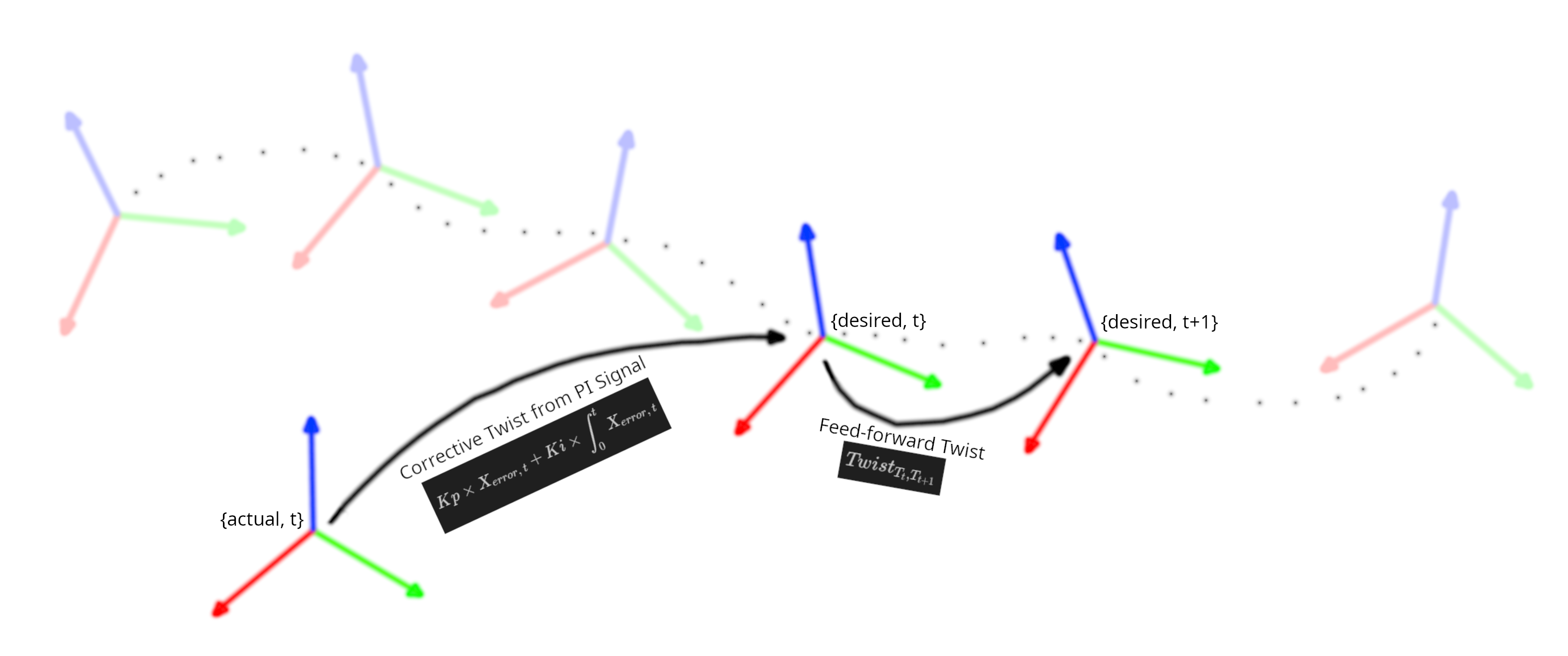
The frame labeled {actual} is the actual pose of the end-effector in the world at time step t and the frames labelled {desired, t} and {desired, t+1} are the desired poses from the trajectory at time stamps t and t+1
As depicted in the image above, the PI terms correct the error between the actual end-effector pose and the desired pose it is supposed to have at timestep \(t\) and the feed forward term is the proactive twist that takes the desired pose at timestep \(t+1\).
The following section goes into further details.
Computing error terms for PI Control
Now that we have the trajectory which defines the end-effector poses for all time \(t \in [0,T]\), we can use this information for trajectory tracking.
At some timestamp \(t\), we first obtain the end-effector pose from the simulator or using the joint states and apply forward kinematics. Let the current end-effector pose be \(T_{ee,\ actual,\ t}\).
We also know the pose that the end-effector should have at timestamp \(t\) which we index from the trajectory which we call \(T_{ee,\ desired,\ t}\). The error is then simply the twist that rotates from \(T_{ee,\ actual,\ t}\) to \(T_{ee,\ desired,\ t}\) and represented in the actual end-effector's frame.
\[T_{ee-desired-in-actual,\ t} = T^{-1}_{ee,\ actual,\ t} T_{ee,\ desired,\ t}\]Then we use the matrix logarithm to map this rigid-body transformation to its derivative (Twist):
\[X_{error,\ t} = MatrixLog(T_{ee-desired-in-actual,\ t})\]We maintain a running sum to integrate the accumulated error.
Computing feed-forward term
The PI error twist simply corrects the error between the actual end-effector pose and the desired end-effector pose at time step \(t\). It is also important that we apply the additional twist that takes the end-effector from the desired pose at timestep \(t\) to the timestep at \(t+1\) so that at the next timestep \(t+1\) the end-effector is as close to the desired pose for \(t+1\) as we can get it.
We call this term the feed-forward component and we compute it just like the PI term, but this time we first compute the twist that takes \(T_{desired,\ t}\) to \(T_{desired,\ t+1}\) represented in the frame at T_{desired,\ t}.
Then we represent that twist in the actual frame of the end-effector, T_{actual,\ t} by transforming it using the adjoint of T^{desired,\ t}_{actual}.
\[X^{T_{t},\ T_{t+1}}_{desired} = SE3toVec(MaxtrixLog((T^{desired,\ t}_{world})^{-1} T^{desired,\ t+1}_{world}))\]Then we change the coordinate frame representation by using the adjoint to get:
\[X^{T_{t},\ T_{t+1}}_{actual} = Adjoint((T^{actual,\ t}_{world})^{-1} T^{desired,\ t}_{world}) X^{T_{t},\ T_{t+1}}_{desired}\]Computing the control twist
These two twists are summed to get the final control twist:
\[\mathcal{V}_{EE,\ t} = Twist_{EE,\ t} = Kp \times X_{error,\ t} + Ki \times \int^{t}_{0} X_{error,\ t} + X^{T_{t},\ T_{t+1}}_{actual}\]Transforming the desired end-effector twists into joint velocities
Now that we have the twist that we want the end-effector to be subjected to, we need to figure out the corresponding joint velocities are to acheieve this twist. This is where the Jacobian matrix comes into play. Simply put, the coloumns of the Jacobian matrix represent the instantaneous contributions of each joint velocity to the end-effector's twist. The mapping looks something like:
\[\mathcal{V} = J \; \dot{q}\]As evidenced by the sub-scripts, the Jacobian is computed for a specific frame and produces the twist caused by the joint velocities as represented in that frame. Since we computed all our twists in the end-effector's frame, we need to construct our Jacbian in the end-effector's frame as well.
Our Jacobian will have two components
\[J = \begin{bmatrix} J_{arm} & J_{chassis} \\ \end{bmatrix}\]The joint screw axes that were used in this implementation are shown in the figure below:
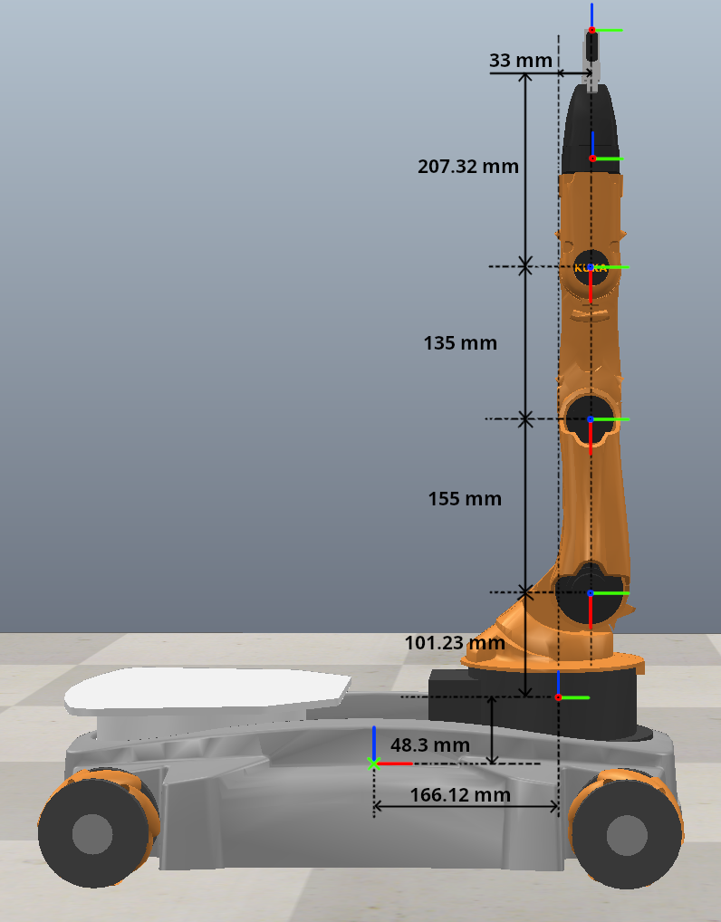
The reference frames on the Kuka robot are as shown in the image with the corresponding offsets between each of them depicted. (Please note, these are different from the coordinate frame placements provided in the Modern Robotics textbook and course assignment to preserve academic integrity.)
The corresponding screw axes for the arm-joints in the end-effector frame are then:
\[\begin{bmatrix} \omega_x & \omega_y & \omega_z & \dot{x} & \dot{y} & \dot{z} \\ 0.0 & 0.0 & 1.0 & -0.033 & -0.0005 & 0.0 \\ 1.0 & 0.0 & 0.0 & 0.0 & -0.49714 & 0.00037 \\ 1.0 & 0.0 & 0.0 & 0.0 & -0.342 & 0.0005 \\ 1.0 & 0.0 & 0.0 & 0.0 & -0.207 & 0.00055 \\ 0.0 & 0.0 & 1.0 & 0.0 & 0.0 & 0.0 \end{bmatrix}\]The jacobian matrices for the arm and the base are computed separately. The jacobian matrix for the arm is computed for each joint. Since we are computing our control twists in the end-effector frame, we want to compute the arm jacobian in the end-effector frame as well.
Since our arm is a 5-DOF arm and twists are 6 dimensional, our jacobian matrix will be a \(6 x 5\) matrix that transforms the joint velocities into the end-effector twist in the end-effector frame.
The ith column of the jacobian for each of our 5 columns can be computed using the following expression:
\[J_{bi}(j_{robot,\ t}) = Ad_{e^{-[\mathcal{B}_{n}]j_{robot, n,\ t}}...e^{-[\mathcal{B}_{i+1}]j_{robot, i+1,\ t}}}(\mathcal{B}_{i})\]for \(i = n-1, ...,1,\) with \(J_{bn} = \mathcal{B}_n\) i.e. the body-jacobian column for the last joint before the end-effector frame is simply the screw-axis for that joint in the end-effector frame.
The matrix transformation called \(Ad\) is the Adjoint transformation. It transforms twists or the normalized screw representations from one frame into the other. So we started out with our home configuration (configuration at which we set our joint angles to be zero) and the screw axes of every joint as represented in the home-configuration end-effector frame. Each screw axis allows us to estimate the twist generated at the end-effector due to the joint rotation at that screw axis. However, this is only valid at the home configuration.
When the configuration of the robot changes, the instantaneous screw axes of every joint also changes (in our case in the instantaneous end-effector frame). This implies that at any given instant, in order to compute the twist at the end-effector due to joint rotations, we first need to transform the screw axis of each joint at the home confiogurastion of the end-effector into the screw aaxis in the end-effector frame at that instant. This is what the Adjoint matrix helps us do.
The Adjoint matrix is computed using the following expression as derived in section adfsdaf of the MR textbook: \([Ad_T] = \begin{bmatrix} R & 0 \\ [p]R & R \end{bmatrix} \in \mathbb{R}^{6 \times 6}\)
The Adjoint is useful when converting the base frame of a twist/screw from one frame into another. The \(p\) translation vector and the rotation matrix \(R\) come from a transformation matrix that represents the transforms between the two coordinate frames.
So the subscript of the Adjoint in this term \(Ad_{e^{-[\mathcal{B}_{n}]j_{robot, n,\ t}}...e^{-[\mathcal{B}_{i+1}]j_{robot, i+1,\ t}}}\) in the Jacobian column computation is simply the matrix-exp products i.e. sequence of joint transforms using the current joint angles that express the relation between the home end-effector frame configuration and the end-effector configuration due to the motion of the joint between joint i and the last joint at the end-effector. The \(R\) and \(p\) components of the result of this transform sequence \(e^{-[\mathcal{B}_{n}]j_{robot, n,\ t}}...e^{-[\mathcal{B}_{i+1}]j_{robot, i+1,\ t}}\) can then be used to compute the Adjoint.
With this we get our \(6 \times 5\) arm jacobian:
\[J_{arm} = \begin{bmatrix} J_{b1} & J_{b2} & J_{b3} & J_{b4} & J_{b5} \end{bmatrix}\]All that's left is to compute the chassis jacobian.
For the chassis jacobian, we need to find an expression that relates wheel velocities to twists in the end-effector frame. The process of deriving this mapping follows a similar process in that we start with a body twist in the robots chassis frame and map it to it's components at the wheel centers. The longitudinal and lateral wheel velocity components are further mapped into the rotation velocity at the wheels. This is done for each wheel. In our case, we have four mecanum wheels on the body of the robot and hence after stacking the relations for each wheel we get a \(4 x 3\) matrix that transforms the body twist into wheel velocities. The chassis jacobian is then given by the inverse of this matrix which maps the wheel velocities to body-twists.
The derivation of these are too lengthy to detail here but are described in detail in sections 13.2 Modelling (derivation of body twist to wheel velocities) and 13.8 Odometry (for the inverse to get the chassis Jacobian).
The transform from body-twist to wheel velocities are given by:
\[\begin{bmatrix} u_1 \\ u_2 \\ u_3 \\ u_4 \end{bmatrix} = \frac{1}{r} \begin{bmatrix} -{l-w} & 1 & -1 \\ {l+w} & 1 & 1 \\ {l+w} & 1 & -1 \\ -{l-w} & 1 & 1 \end{bmatrix} \begin{bmatrix} \omega_z \\ v_x \\ v_y \end{bmatrix}\]Where \(l\) is the half wheelbase of the robot and w is the half width of the robot, see Figure 13.5 in the Modern Robotics textbook.
And it's pseudo-inverse then is:
\[\begin{bmatrix} \omega_z \\ v_x \\ v_y \end{bmatrix} = \frac{r}{4} \begin{bmatrix} -\frac{1}{l+w} & \frac{1}{l+w} & \frac{1}{l+w} & -\frac{1}{l+w} \\ 1 & 1 & 1 & 1 \\ -1 & 1 & -1 & 1 \end{bmatrix} \begin{bmatrix} \dot{u_1} \\ \dot{u_2} \\ \dot{u_3} \\ \dot{u_4} \end{bmatrix}\]We re-write this to apply to 6-DOF twists, so
\[\mathcal{V}_b = \begin{bmatrix} \omega_x \\ \omega_y \\ \omega_z \\ v_x \\ v_y \\ v_z \end{bmatrix} = \begin{bmatrix} 0 & 0 & 0 & 0 \\ 0 & 0 & 0 & 0 \\ -\frac{1}{l+w} & \frac{1}{l+w} & \frac{1}{l+w} & -\frac{1}{l+w} \\ 1 & 1 & 1 & 1 \\ -1 & 1 & -1 & 1 \\ 0 & 0 & 0 & 0 \end{bmatrix} \begin{bmatrix} \dot{u_1} \\ \dot{u_2} \\ \dot{u_3} \\ \dot{u_4} \end{bmatrix}\]Here
\[J_{chassis} = \begin{bmatrix} 0 & 0 & 0 & 0 \\ 0 & 0 & 0 & 0 \\ -\frac{1}{l+w} & \frac{1}{l+w} & \frac{1}{l+w} & -\frac{1}{l+w} \\ 1 & 1 & 1 & 1 \\ -1 & 1 & -1 & 1 \\ 0 & 0 & 0 & 0 \end{bmatrix}\]Stacking the arm-jacobian and the chassis jacobian together now gives us the complete transformation as below:
\[\mathcal{V}_b = \begin{bmatrix} J_{arm} & J_{chassis} \end{bmatrix} \begin{bmatrix} \dot{\theta_1} \\ \dot{\theta_2} \\ \dot{\theta_3} \\ \dot{\theta_4} \\ \dot{\theta_5} \\ \dot{u_1} \\ \dot{u_2} \\ \dot{u_3} \\ \dot{u_4} \end{bmatrix}\]To therefore get the joint velocities, we simply take the pseudo-inverse of this Jacobian to get the relation:
\[\begin{bmatrix} \dot{\theta_1} \\ \dot{\theta_2} \\ \dot{\theta_3} \\ \dot{\theta_4} \\ \dot{\theta_5} \\ \dot{u_1} \\ \dot{u_2} \\ \dot{u_3} \\ \dot{u_4} \end{bmatrix} = \begin{bmatrix} J_{arm} & J_{chassis} \end{bmatrix}^{\dagger}_{j_{robot,\ t}} \mathcal{V}_b\]Applying joint velocities to the simulated robot's joints
The joint velocities obtained above are then simply fed to Coppeliasim and the simulation stepped for the set timestep to get the next state of the robot.
In this implementation, CoppeliaSim was set to run in client stepped mode so that we can ignore any performance deviations of the controller from the simulation timestep and simply focus on the logical implementation.